10 Exciting Beginner Machine Learning Projects of 2022

Table of Contents
- Zillow Home Value Prediction
- Article Recommendation System
- Iris Flowers Classification
- Instagram Reach Analysis and Prediction
- BigMart Sales Prediction
- Stock Prices Predictor using TimeSeries
- Waiter Tips Analysis & Prediction
- Music Recommendation System
- Covid-19 Deaths Prediction
- Stress Detection
- Helpful Links
Zillow Home Value Prediction
Zestimate is a tool that provides the worth of the house based on various attributes like public data, sales data, etc. Zestimate has information of more than 97 million homes. Zestimate is the first step to analyze the worth of a house or to check if the value has been appraised or not after newly upgrading your home, or maybe you just want to refinance it. The algorithm behind Zestimate gets its data 3 times a week, on the basis of comparable sales and publicly available data.
Building a model to improve the Zestimate residual error which is called “log error” which is the difference between the log of Zestimate price and the log of the actual sales price
log error = log(Zestimate) — log(SalePrice)
Machine Learning project Workflow:
1. Import Libraries and Loading Dataset
Here you will be using python, opendatasets, pandas, seaborn, matplotlib, ploitly, geopands, sklearn, etc.
2. Exploratory Data Analysis
- Look at missing values
- Illustrate distribution and outliers
- Analyze
3. Fix and clean the data
You'll find around 35 columns with ~30% missing values. Data cleaning is one of the critical steps in machine learning techniques used to appropriately clean the data.
4. Data splitting
5. Baseline model training
3 models: a hard coded model that only predicts average, Linear Regression, and Decision Tree models.
6. Feature engineering & Feature selection
7. Data Pre-processing
8. Robust model Training and Hyperparameter tuning
You can train the data on models such as SkLearn ensemble Tree-based models Random Forest, Gradient Boosting, ExtraTree, and also models such as LightGBM, Catboost.
Check out this Github here for the full code and explantion
Article Recommendation System
There are two types of recommendation systems. Collaborative filtering and content-based filtering.
Machine Learning project Workflow:
1. Import Libraries and Loading Dataset
You'd use numpy, pandas, gdown, fastai, motplotlib, zipfile, time, google.colab, etc.
import matplotlib.pyplot as plt
import numpy as np
import pandas as pd
import gdown
from fastai.vision import *
from fastai.metrics import accuracy, top_k_accuracy
from annoy import AnnoyIndex
import zipfile
import time
from google.colab import drive
%matplotlib inline
2. Getting images from Google Drive
# get the images
root_path = './'
url = 'https://drive.google.com/uc?id=1j5fCPgh0gnY6v7ChkWlgnnHH6unxuAbb'
output = 'img.zip'
gdown.download(url, output, quiet=False)
with zipfile.ZipFile("img.zip","r") as zip_ref:
    zip_ref.extractall(root_path)
3. Data preparation and cleaning
4. Retrieve image embed with FastAI
5. Testing the system
Talk a look at thecleverprogrammer for the code and explanation of recommendation systems in ML.
Iris Flowers Classification
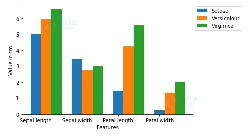
Iris flower classification is a very popular machine learning project. The iris dataset contains three classes of flowers, Versicolor, Setosa, Virginica, and each class contains 4 features, ‘Sepal length’, ‘Sepal width’, ‘Petal length’, ‘Petal width’. The aim of the iris flower classification is to predict flowers based on their specific features.
Machine Learning project Workflow:
1. Importing the libraries
You'll be using numpy, matplotlib, seaborn, pandas, and scikit-learn. You can find a source code of the iris flower classification for download here with opencv.
2. Analyze and visualize the dataset
sns.pairplot(df, hue='Class_labels')
# Separate features and target
data = df.values
X = data[:,0:4]
Y = data[:,4]
# Calculate average of each features for all classes
Y_Data = np.array([np.average(X[:, i][Y==j].astype('float32')) for i in range (X.shape[1])
 for j in (np.unique(Y))])
Y_Data_reshaped = Y_Data.reshape(4, 3)
Y_Data_reshaped = np.swapaxes(Y_Data_reshaped, 0, 1)
X_axis = np.arange(len(columns)-1)
width = 0.25
plt.bar(X_axis, Y_Data_reshaped[0], width, label = 'Setosa')
plt.bar(X_axis+width, Y_Data_reshaped[1], width, label = 'Versicolour')
plt.bar(X_axis+width*2, Y_Data_reshaped[2], width, label = 'Virginica')
plt.xticks(X_axis, columns[:4])
plt.xlabel("Features")
plt.ylabel("Value in cm.")
plt.legend(bbox_to_anchor=(1.3,1))
plt.show()
3. Model training
Here you want to split the whole data into training and testing datasets. The testing dataset will be used to check the accuracy of the model. You feed the training dataset into the algorithm.
4. Model evaluation
Now you predict the classes from the test dataset from the trained model and check the accuracy score of the predicted classes.
5. Testing the model
Instagram Reach Analysis and Prediction
Here is a dataset you can use for this project. There's even a paper on this topic found here.
Machine Learning project Workflow:
1. Building the dataset
You'll be using libraries such as pandas, numpy, matplotlib, seaborn, plotly, wordcloud, sklearn, etc.
2. The scraper
Instagram's API has a limit of 60 requests/hour to their backend servers. You'll want a scraper to linearly scan the latest posts of a user, then opens each post to retrieve more granular information related to each image.
3. Dataset analysis
If you are using the dataset provided above (here's the link), then let's start from here.
import pandas as pd
import numpy as np
import matplotlib.pyplot as plt
import seaborn as sns
import plotly.express as px
from wordcloud import WordCloud, STOPWORDS, ImageColorGenerator
from sklearn.model_selection import train_test_split
from sklearn.linear_model import PassiveAggressiveRegressor
Run this to check if the dataset contains null values:
data.isnull().sum()
And this should be the output:
Impressions       1
From Home         1
From Hashtags     1
From Explore      1
From Other        1
Saves             1
Comments          1
Shares            1
Likes             1
Profile Visits    1
Follows           1
Caption           1
Hashtags          1
dtype: int64
When you get null values, you'll want to drop them by running data = data.dropna(). Next:
data = pd.read_csv("Instagram.csv", encoding = 'latin1')
print(data.head())
You'll get something like this...
Impressions From Home From Hashtags From Explore From Other Saves \
0 3920.0 2586.0 1028.0 619.0 56.0 98.0
1 5394.0 2727.0 1838.0 1174.0 78.0 194.0
2 4021.0 2085.0 1188.0 0.0 533.0 41.0
3 4528.0 2700.0 621.0 932.0 73.0 172.0
4 2518.0 1704.0 255.0 279.0 37.0 96.0
Comments Shares Likes Profile Visits Follows \
0 9.0 5.0 162.0 35.0 2.0
1 7.0 14.0 224.0 48.0 10.0
2 11.0 1.0 131.0 62.0 12.0
3 10.0 7.0 213.0 23.0 8.0
4 5.0 4.0 123.0 8.0 0.0
Caption \
0 Here are some of the most important data visua...
1 Here are some of the best data science project...
2 Learn how to train a machine learning model an...
3 Heres how you can write a Python program to d...
4 Plotting annotations while visualizing your da...
Hashtags
0 #finance #money #business #investing #investme...
1 #healthcare #health #covid #data #datascience ...
2 #data #datascience #dataanalysis #dataanalytic...
3 #python #pythonprogramming #pythonprojects #py...
4 #datavisualization #datascience #data #dataana...
4. Visualizing data
To get different plots, you can run:
plt.figure(figsize=(10, 8))
plt.title("Distribution of Impressions From Hashtags")
sns.distplot(data['From Hashtags'])
plt.show()
and/or
home = data["From Home"].sum()
hashtags = data["From Hashtags"].sum()
explore = data["From Explore"].sum()
other = data["From Other"].sum()

labels = ['From Home','From Hashtags','From Explore','Other']
values = [home, hashtags, explore, other]

fig = px.pie(data, values=values, names=labels, title='Impressions on Instagram Posts From Various Sources', hole=0.5)
fig.show()
and/or
text = " ".join(i for i in data.Caption)
stopwords = set(STOPWORDS)
wordcloud = WordCloud(stopwords=stopwords, background_color="white").generate(text)
plt.style.use('classic')
plt.figure( figsize=(12,10))
plt.imshow(wordcloud, interpolation='bilinear')
plt.axis("off")
plt.show()
5. Prediction Model
You'll want to split the data into training and test sets.
x = np.array(data[['Likes', 'Saves', 'Comments', 'Shares', 'Profile Visits', 'Follows']])
y = np.array(data["Impressions"])
xtrain, xtest, ytrain, ytest = train_test_split(x, y,
                                                test_size=0.2,
                                                random_state=42)
Then predict the reach of an Instagram post by giving inputs into the ML model.
Check thecleverprogrammer for the full code.
BigMart Sales Prediction
Machine Learning project Workflow:
1. Exploratory data analysis (EDA)
- Distribution of target variables
- Numerical predictors
- Categorical predictors
- Distribution of variables
- Bivariate analysis
2. Data Pre-processing
- Looking for missing values
- Inputting missing values
- Normalization of dataset for improved results
3. Feature engineering
- Creating broad categories
- Modifying categories
4. Building a model
- fit(x, y)
- predict(x)
- test_size=0.2
- n_estimators=50
- learning_rate = 0.1
- random_state = default

BigMart Outlet Sales Prediction. The data scientists at BigMart have… | by Precious Kolawole | Medium
Precious Kolawole ・ ・
 precillieo.Medium
 precillieo.Medium
Stock Prices Predictor using TimeSeries

where P1 to Pn are n immediate data points that occur before the present, so to predict the present data point, we take the SMA of the size n (meaning that we see up to n data points in the past).

where Pt is the price at time t and k is the weight given to that data point. EMA(t-1) represents the value computed from the past t-1 points. Clearly, this would perform better than a simple MA. The weight k is computed as k = 2/(N+1).
Looking closely at the formula of RMSE, we can see how we will be able to consider the difference (or error) between the actual (At) and predicted (Ft) price values for all N timestamps and get an absolute measure of error.

On the other hand, MAPE looks at the error concerning the true value – it will measure relatively how far off the predicted values are from the truth instead of considering the actual difference. This is a good measure to keep the error ranges in check if we deal with too large or small values. For instance, RMSE for values in the range of 10e6 might blow out of proportion, whereas MAPE will keep error in a fixed range.

Download stock data from yahoo
Machine Learning project Workflow:
1. Loading the datasets and libraries
You'll be using pandas, matplotlib, datetime, numpy, sklearn, etc.
2. Data Preprocessing
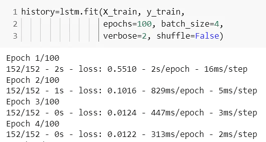
You'll have 757 data samples in the dataset. An LSTM model requires a window or timestep of data in each training step. For example, each 10 data samples to predict the 10th one.
3. Train and test sets
Here, you want to split the data into training and testing sets.
4. Building the LSTM model
5. Performance Evaluation on test set
To get better results with the same dataset, you add another LSTM layer and increase the number of LSTM units per layer.
Check projectpro.io for the full code and explanation.
Waiter Tips Analysis & Prediction
Tipping waiters for serving food depends on many factors like the type of restaurant, how many people you are with, how much amount you pay as your bill, etc. Waiter Tips analysis is one of the popular data science case studies where we need to predict the tips given to a waiter for serving the food in a restaurant.
Download the dataset here
Machine Learning project Workflow:
1. Import libraries and dataset
import pandas as pd
import numpy as np
import plotly.express as px
import plotly.graph_objects as go

data = pd.read_csv("tips.csv")
print(data.head())
2. Data Analysis
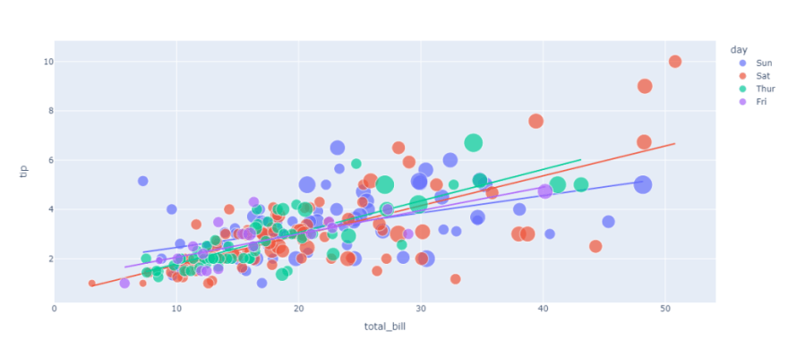
figure = px.scatter(data_frame = data, x="total_bill",
                    y="tip", size="size", color= "day", trendline="ols")
figure.show()
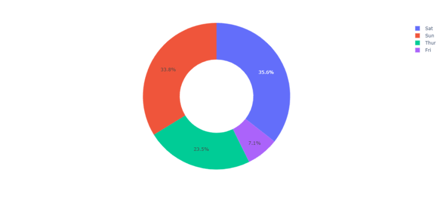
figure = px.pie(data, values='tip', names='day',hole = 0.5)
figure.show()
3. Prediction Model
You'll want to format your data first:
data["sex"] = data["sex"].map({"Female": 0, "Male": 1})
data["smoker"] = data["smoker"].map({"No": 0, "Yes": 1})
data["day"] = data["day"].map({"Thur": 0, "Fri": 1, "Sat": 2, "Sun": 3})
data["time"] = data["time"].map({"Lunch": 0, "Dinner": 1})
data.head()
Then split your data into training and test sets:
x = np.array(data[["total_bill", "sex", "smoker", "day", "time", "size"]])
y = np.array(data["tip"])

from sklearn.model_selection import train_test_split
xtrain, xtest, ytrain, ytest = train_test_split(x, y,
                                                test_size=0.2,
                                                random_state=42)
4. Training the model
You can use LinearRegression from sklearn here:
from sklearn.linear_model import LinearRegression
model = LinearRegression()
model.fit(xtrain, ytrain)
Check out thecleverprogrammer for the full code and explanation.
Music Recommendation System
See codespeedy for a step-by-step guideline
Covid-19 Deaths Prediction
Governments and other legislative bodies rely on these kinds of machine learning predictive models and ideas to suggest new policies and assess the effectiveness of applied policies.
Machine Learning project Workflow:
1. Import the libraries and dataset
import pandas as pd
import numpy as np
import matplotlib.pyplot as plt
import plotly.express as px

from fbprophet import Prophet
from sklearn.metrics import r2_score

plt.style.use("ggplot")

df0 = pd.read_csv("CONVENIENT_global_confirmed_cases.csv")
df1 = pd.read_csv("CONVENIENT_global_deaths.csv")
2. Data preparation
Combine the above dataset and get a visualization of the data to see what you are working with.
3. Data Visualization
fig = px.choropleth(world.dropna(),locations="Alpha3", color="Cases Range", projection="mercator", color_discrete_sequence ["white","khaki","yellow","orange","red"])
fig.update_geos(fitbounds="locations", visible=False)
fig.update_layout(margin={"r":0,"t":0,"l":0,"b":0})
fig.show()
4. Prediction for the next 30 days
Use Facebook prophet model here
model = Fbprophet()
model.fit(df_fb)
model.forecast(30,"D")
model.R2()

forecast = model.df_forecast[["ds","yhat_lower","yhat_upper","yhat"]].tail(30).reset_index().set_index("ds").drop("index",axis=1)
forecast["yhat"].plot(marker=".",figsize=(10,5))
plt.fill_between(x=forecast.index, y1=forecast["yhat_lower"], y2=forecast["yhat_upper"],color="gray")
plt.legend(["forecast","Bound"],loc="upper left")
plt.title("Forecasting of Next 30 Days Cases")
plt.show()
Check thecleverprogrammer for the full code and explanation.
Stress Detection
Stress, anxiety, and depression are threatening the mental health of people. Every person has a reason for having a stressful life. Many content creators have come forward to create content to help people with their mental health. Many organizations can use stress detection to find which social media users are stressed to help them quickly.
Machine Learning project Workflow:
1. Import the libraries and dataset
import pandas as pd
import numpy as np
data = pd.read_csv("stress.csv")
print(data.head())
2. Visualize the dataset
import matplotlib.pyplot as plt
from wordcloud import WordCloud, STOPWORDS, ImageColorGenerator
text = " ".join(i for i in data.text)
stopwords = set(STOPWORDS)
wordcloud = WordCloud(stopwords=stopwords,
                      background_color="white").generate(text)
plt.figure( figsize=(15,10))
plt.imshow(wordcloud, interpolation='bilinear')
plt.axis("off")
plt.show()
3. Building the model
The label column in this dataset contains labels as 0 and 1. 0 means no stress, and 1 means stress.
data["label"] = data["label"].map({0: "No Stress", 1: "Stress"})
data = data[["text", "label"]]
print(data.head())
4. Splitting the dataset
from sklearn.feature_extraction.text import CountVectorizer
from sklearn.model_selection import train_test_split

x = np.array(data["text"])
y = np.array(data["label"])

cv = CountVectorizer()
X = cv.fit_transform(x)
xtrain, xtest, ytrain, ytest = train_test_split(X, y,
                                                test_size=0.33,
                                                random_state=42)
5. Training the model
from sklearn.naive_bayes import BernoulliNB
model = BernoulliNB()
model.fit(xtrain, ytrain)
6. Testing the model
user = input("Enter a Text: ")
data = cv.transform([user]).toarray()
output = model.predict(data)
print(output)
Check thecleverprogrammer for the full code and explanation
Helpful Links
- ALL files of thecleverprogrammer
- 285+ Machine Learning Projects with Python
- Ten Projects for Beginners to Get Started
- Top 10 Machine Learning Projects for Beginners in 2022
- PyTorch
Happy coding!


